Find text at end of a string by finding last delimiter

You want to find text at the end a string, such as a path or URL. You want to find all the text after the last slash say. This formula will do it.

=RIGHT(A1,LEN(A1)-FIND("@",SUBSTITUTE(A1,"/","@",LEN(A1)-LEN(SUBSTITUTE(A1,"/",""))),1))

Autosized named ranges in Excel

Named ranges are great to identify the location of data tables in Excel. However when new data is added, the named range need to be adjusted. Data Connections and the Table feature dynamically size named ranges as required. But if that does not suit your requirements or the data is updated by hand, updating the named range is awkward and likely to be forgotten.

Hence a formula to build a dynamically sized named range in Excel. Instead of entering the traditional range use variations of this formula to define the range.

=OFFSET('Sheet1'!$A$2,0,0,COUNTA('Sheet1'!$A:$A)-1,COUNTA('Sheet1'!$2:$2))

A formula to change the colour of a worksheet tab

Came across this article to create a formula to change the tab colour of a worksheet.

In summary it is

Function ChangeTabColor(sht As String, RED_Color As Integer, GREEN_Color As Integer, BLUE_Color As Integer)

With ActiveWorkbook.Sheets(sht).Tab

.Color = RGB(RED_Color, GREEN_Color, BLUE_Color)

End With

End Function

For example, entering this formula in a cell will turn the tab on Sheet1 red.

=ChangeTabColor(“Sheet1”,255,0,0)

Excel Camera – for creating dashboard and cross checks

Excel has a ‘hidden’ feature called a Camera. It allows you to select a range of cells, or chart and copy and paste it somewhere else. It will then update as changes are made to the source.

This is especially useful as the copy may be trimmed of unnecessary information, such a pivot table headings. It can also be stretched and rotated like a graphic, all quite simply.

We start by adding the Camera tool to the quick access tool bar because it is not available on the ribbon.

• Select the File Tab, then select
• Select the Quick Access Toolbar.
• In the Choose Commands From drop-down menu, select Commands Not in the Ribbon.
• Scroll down the list of commands and find Camera.
• Select Add, and then select Camera.

Thanks to Sage Intelligence for the tip and further examples and a tutorial if required.

Lookup data in Excel using multiple criteria

You can lookup data that meets multiple criteria and overcome the limitations of the Vlookup, thus saving you time and making your process more efficient.

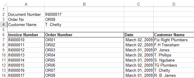
Follow the example below, as I explain how to use the invoice number and order number to extract the customer’s name.

Applies To: Microsoft^® Excel^® 2010 and 2013.

1.Place the cursor in cell B4 and enter the following formula:

=INDEX(Data_Source,MATCH(B2&B3,Invoice_Number&Order_Number,0),4)

• To display the data range for the entire table, place the cursor after “=INDEX( “.
  • Press F3 and select Data_Source.
• B2&B3 represents the invoice number and order number respectively.
• To display the data range for the invoice number, place the cursor after “MATCH(B2&B3,”.
  • Press F3 and select Invoice_Number.
• To display the data range for the order number ,place the cursor after “MATCH(B2&B3,Invoice_Number&”
  • Press F3 and select Order_Number.
• 0 means an exact match should be found.
• 4 is the position of the customer name field within the main table range.

2.Press CTRL +SHIFT +ENTER because it is an array formula.

By using this formula you can lookup data with multiple criteria. It will let you analyze your data quicker and help save time! This will enable you to analyze data quickly.

Thanks to Sage Intelligence for this tip, they also have an example workbook.

Excel Number format

In the good old days Excel had a nice negative number format that followed accounting conventions by placing negative numbers in brackets. After all this is the presentation method for financial statements in Australia for many years.

To re-create the number format use the follow custom number format.

#,##0.00_);(#,##0.00);-??_)

The bit a the end is to align the dash with the dollars column not the cents.

Update: Using ? instead of _0 for a blank digit

Mathematically convert Date to Fiscal Year

Problem

Date are expressed as  Day Month Year, Many systems allow you to extract the Year. Most often a client requires the Fiscal Year not Calendar Year.

So late 2015 should be Fiscal year 2016 and Early 2016 should also be 2016 while late 2016 should be 2017 assuming a 30 June year end.

Solution

This works for 1 July to 30 June Fiscal Year.

Extract the Year and Add the Month divided by 7 as an Integer.

=YEAR(A3)+INT(MONTH(A3)/7)

Excel number format that prompts for a user response

Excel spreadsheets are often used for more than calculating numbers. Spreadsheets are often used to collect information as well.

This raises a problem of how to let the person providing the information know where the information is to be entered. Many approaches include using colour to indicate cells requiring a response. This may be extended to use conditional formatting to change the colour once the entry changes. Other approaches include arrows, comments and other labels.

One other way is to put the prompt text in the cell itself. This will usually result in errors in formula that link to the cell as text does not work with numbers.

An alternative to typing in text is to make a number, usually zero, look like text.

Excel allows custom number formats, which include how many decimal places, commas, dates, time and others. There are four parts, The first part is for positive numbers, then negative numbers, then the format of zero and lastly the format of text. After the first part each is optional, but they must be in this order.

So why not make zero look like the text to prompt for input.

The following number format will display numbers, but replaces the number zero with the words “Entry Required”.

0;(0);"Entry Required"

Now fill the areas asking for information with zero, and the words  “Entry Required” will appear, but other formulas will read this a zero.

Of course this may create other issues such as divide by zero errors and you should still have a check that all the data has been entered when returned.

If zero is a valid response you could use positive or negative number formats to do the same.

For example if you asked, how many staff are there? A valid answer might be zero, but is unlikely to be negative. You could use the following number format

0;"Entry Required";0

Now enter -1 and the text “Entry Required” will appear. Just remember that the worksheet should ignore negative numbers.

Custom number formats are a robust way of asking for information and getting it in the correct place.

Looking up values in Excel

While the Microsoft Excel functions LOOKUP and its partners VLOOKUP and HLOOKUP, are especially useful in finding information in tables in spreadsheets, they have their problems.

LOOKUP requires that the list be sorted, otherwise it may find the wrong value.

VLOOKUP and HLOOKUP, can find a value in an unsorted list, but are slow is large tables (for example, I built a table of 65,000 lookups finding values in three tables of 500 each , and Excel took 45 sec to recalculate).

Using INDEX with MATCH is much faster (the same example I built of 65,000 lookups finding values in tables of 500 took 6 secs to recalculate). Also INDEX with MATCH allows a horizontal and vertical lookup at the same time.

The syntax is

=INDEX(array,row_num,column_num)

Array is the range to find the values in and then replace Row and Column with Match and the offset. 

At this point I should point out a robust replacement for the offset. If looking up values in column A to find the value in column B, the simple approach would be to use the offset 2. A better approach is the function COLUMNS(A:B). The result is still 2. If you insert a column between A and B, Excel will not change 2 to 3, but it will change (A:B) to (A:C), with the new result of 3, so it is more robust. Also for us humans, when reading the formula, we know the result is in Column B or C, we don’t have to count the number of columns, much more useful in large worksheets.

So a replacement for the simple

=VLOOKUP(A1,D:E,2,FALSE)

is

=INDEX(D:E,MATCH(A1,D:D,0),COLUMNS(D:E))

This is more robust, if you move columns E it will continue to work, and is much quicker for Excel.

INDEX can also do the two-way lookup, something that the Lookups don’t. For example

=INDEX(D:Z,MATCH(A1,D:D,0),MATCH(A2,1:1,0))

will match A1 in the first column, and A2 in the first Row and return the value at the intersection of the two.